
Bayesian Regression
greta and Stan go for a walk
I have been working on my Bayesian statistics skills recently. In particular, I have been reading David Robinson’s lovely Introduction to Empirical Bayes: Examples from Baseball Statistics and watching Rasmus Bååth’s delightful three-part Video Introduction to Bayesian Data Analysis, notable amongst other videos, courses, and textbooks. I have much yet to learn, but my past experience with statistics has taught me that I understand concepts most thoroughly by actually implementing them. Thus, this post is a neophyte’s pass at implementing Bayesian regression with some powerful (and complicated) tools. As such, it almost certainly contains some inaccuracies and statistical failings. (If you notice them, please let me know!) Nonetheless, I present it with the motivation that seeing variations in others’ implementations of code helps us see more options and pick better ones when writing our own.
The example
What follows is two implementations of Bayesian linear regression with Stan and greta, two interfaces for building and evaluating Bayesian models. The example is adapted from the Stan (§9.1, p. 123 of the PDF) and greta docs.
It is a very simple linear regression of a single variable. Its frequentist equivalent would be
lm(mpg ~ wt, mtcars)
#>
#> Call:
#> lm(formula = mpg ~ wt, data = mtcars)
#>
#> Coefficients:
#> (Intercept)           wt
#>      37.285       -5.344
or visually,
library(ggplot2)
theme_set(hrbrthemes::theme_ipsum_rc())

ggplot(mtcars, aes(wt, mpg)) +
    geom_point() +
    geom_smooth(method = "lm")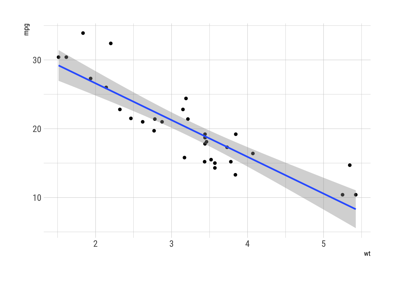
The tools
Stan
Stan is a DSL for implementing Bayesian models. The model is composed in Stan, and then compiled and called from an interface in another language—in R, the rstan package. The Stan code compiles to C++, and rstan makes parallelization across chains simple.
It has its own shirts.
greta
greta is an R package by Nick Golding that implements MCMC sampling in TensorFlow, and can thus run on GPUs and scale well, provided the appropriate hardware and drivers. It is built on top of RStudio’s tensorflow package.
It does not have shirts, as far as I am aware, but does have a nice logo that would make a handsome hex sticker.
The code
Stan
The Stan model has to be composed in, well, Stan. This can be in a separate
file or a string, but I find the former usually too disconnected from the rest
of the code and the latter a magnet for typos. The better solution in my
attempts thus far is to implement the model in an RMarkdown code chunk with an
output.var parameter set. When the chunk is run, the model is compiled and
assigned to an R object with the supplied name. Code highlighting, completion,
and so on work as usual.
Stan is declarative imperative1, with
chunks to define input data, parameters, the model, and more as necessary.
Keeping it very simple, we will supply
n, a number of observations,x, our single feature (a vector of lengthn), andy, our output (another vector of lengthn).
The model will calculate
beta0, the y intercept,beta1, the slope, andsigma, the standard deviation of y.
While we could supply informative priors by adding lines like
beta0 = normal(30, 2);, we will instead leave it blank, so Stan will use a
uniform prior, determining a plausible range by running lots of warm-up
iterations.
Our model is just a line. We assume our outputs are normally distributed, with
a mean defined by the line, and a standard deviation parameterized by sigma.
All together, and set to output to an R variable called model_stan:
data {
    int<lower=0> n;
    vector[n] x;
    vector[n] y;
}

parameters {
    real beta0;
    real beta1;
    real<lower=0> sigma;
}

model {
    y ~ normal(beta0 + beta1*x, sigma);
}
Compiling takes about 40 seconds on my computer. It also produces 15 warnings that
warning: pragma diagnostic pop could not pop, no matching push [-Wunknown-pragmas] #pragma clang diagnostic pop
but apparently they’re harmless,
so I set message=FALSE.
To run the model, we just load rstan and call sampling on the compiled model,
supplying the data. I set the algorithm to Hamiltonian Monte Carlo and the
number of chains to 1 so as to compare more equally with greta.
library(rstan)

draws_stan <- sampling(model_stan,
                       data = list(n = nrow(mtcars),
                                   x = mtcars$wt,
                                   y = mtcars$mpg),
                       seed = 47,
                       algorithm = "HMC",
                       chains = 1)
#>
#> SAMPLING FOR MODEL 'mtcars' NOW (CHAIN 1).
#>
#> Gradient evaluation took 2.3e-05 seconds
#> 1000 transitions using 10 leapfrog steps per transition would take 0.23 seconds.
#> Adjust your expectations accordingly!
#>
#>
#> Iteration:    1 / 2000 [  0%]  (Warmup)
#> Iteration:  200 / 2000 [ 10%]  (Warmup)
#> Iteration:  400 / 2000 [ 20%]  (Warmup)
#> Iteration:  600 / 2000 [ 30%]  (Warmup)
#> Iteration:  800 / 2000 [ 40%]  (Warmup)
#> Iteration: 1000 / 2000 [ 50%]  (Warmup)
#> Iteration: 1001 / 2000 [ 50%]  (Sampling)
#> Iteration: 1200 / 2000 [ 60%]  (Sampling)
#> Iteration: 1400 / 2000 [ 70%]  (Sampling)
#> Iteration: 1600 / 2000 [ 80%]  (Sampling)
#> Iteration: 1800 / 2000 [ 90%]  (Sampling)
#> Iteration: 2000 / 2000 [100%]  (Sampling)
#>
#>  Elapsed Time: 0.23787 seconds (Warm-up)
#>                0.034739 seconds (Sampling)
#>                0.272609 seconds (Total)

draws_stan
#> Inference for Stan model: mtcars.
#> 1 chains, each with iter=2000; warmup=1000; thin=1;
#> post-warmup draws per chain=1000, total post-warmup draws=1000.
#>
#>         mean se_mean   sd   2.5%    25%    50%    75%  97.5% n_eff Rhat
#> beta0  37.02    0.08 1.53  34.08  36.02  36.96  37.99  40.10   402 1.00
#> beta1  -5.27    0.02 0.46  -6.15  -5.57  -5.25  -4.96  -4.43   389 1.00
#> sigma   3.10    0.01 0.36   2.46   2.86   3.08   3.31   3.94  1000 1.00
#> lp__  -51.08    0.10 1.28 -54.51 -51.61 -50.73 -50.17 -49.65   179 1.01
#>
#> Samples were drawn using HMC(diag_e) at Fri May  4 19:52:44 2018.
#> For each parameter, n_eff is a crude measure of effective sample size,
#> and Rhat is the potential scale reduction factor on split chains (at
#> convergence, Rhat=1).
Since this is a very small model, it runs nearly instantaneously (0.26 seconds). The print methods of the call and resulting model are nicely informative. It looks good, but let’s check the diagnostic plots:
plot(draws_stan)
#> ci_level: 0.8 (80% intervals)
#> outer_level: 0.95 (95% intervals)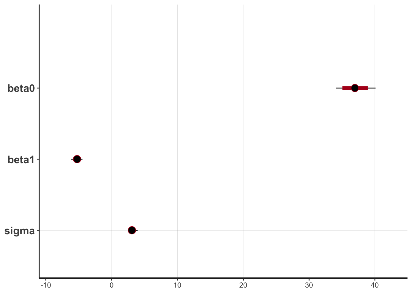
traceplot(draws_stan)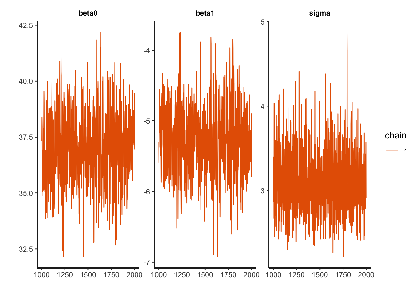
The intercept is moving more than the slope or standard deviation, which is reasonable considering the dimensions. The data is not totally linear (it could be better fit with a quadratic function), but the traceplots are fuzzy caterpillars, so it seems all is well.
Let’s extract the data and plot:
draws_stan_df <- as.data.frame(draws_stan)

ggplot(draws_stan_df, aes(beta0, beta1, color = sigma)) +
    geom_point(alpha = 0.3) +
    geom_density2d(color = "gray30") +
    scale_color_viridis_c(option = "plasma") +
    labs(title = "Stan parameter space")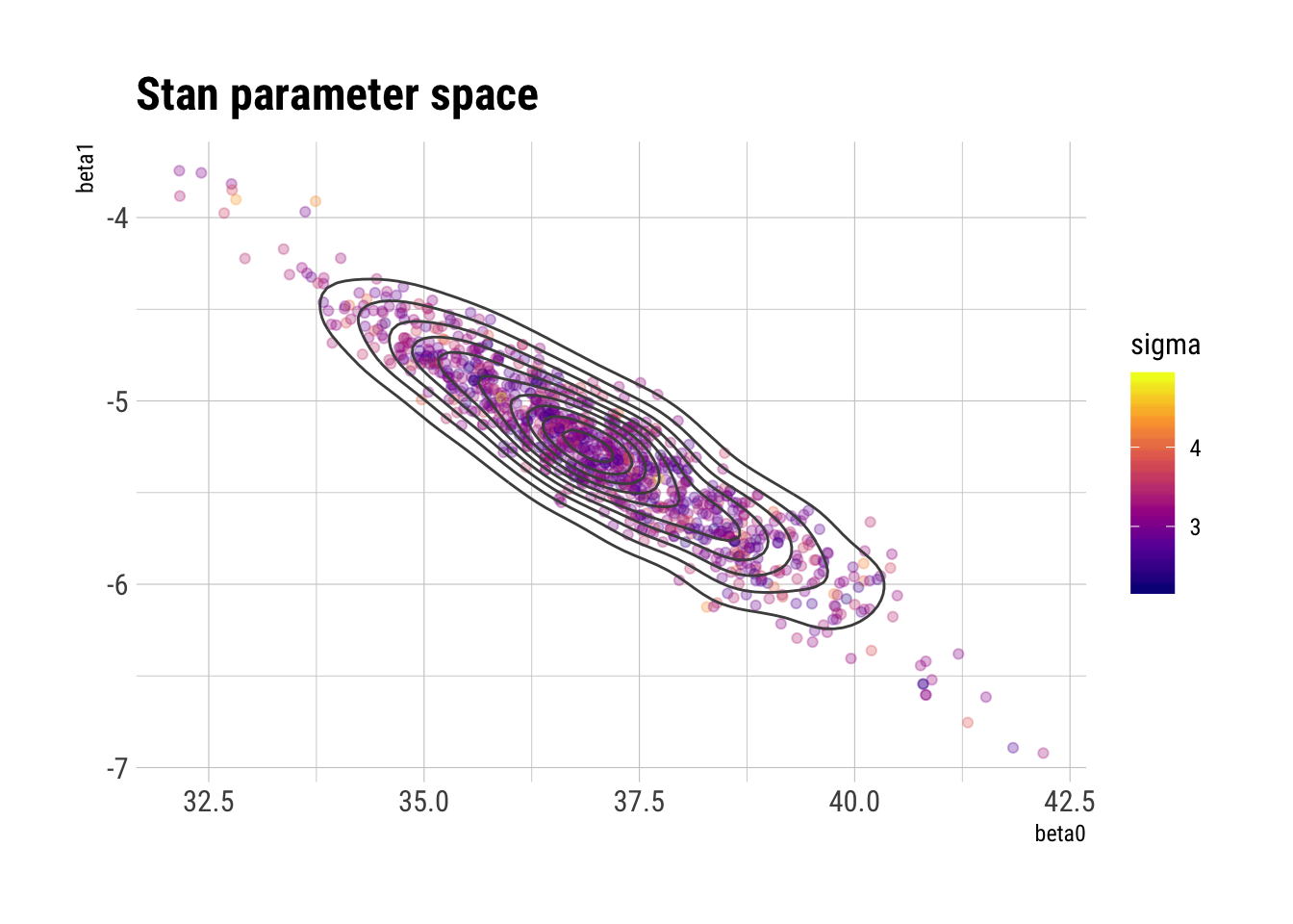
ggplot(mtcars, aes(wt, mpg)) +
    geom_point() +
    geom_abline(aes(intercept = beta0, slope = beta1), draws_stan_df,
                alpha = 0.1, color = "gray50") +
    geom_abline(slope = mean(draws_stan_df$beta1),
                intercept = mean(draws_stan_df$beta0),
                color = "blue", size = 1) +
    labs(title = "Bayesian regression on mtcars via Stan")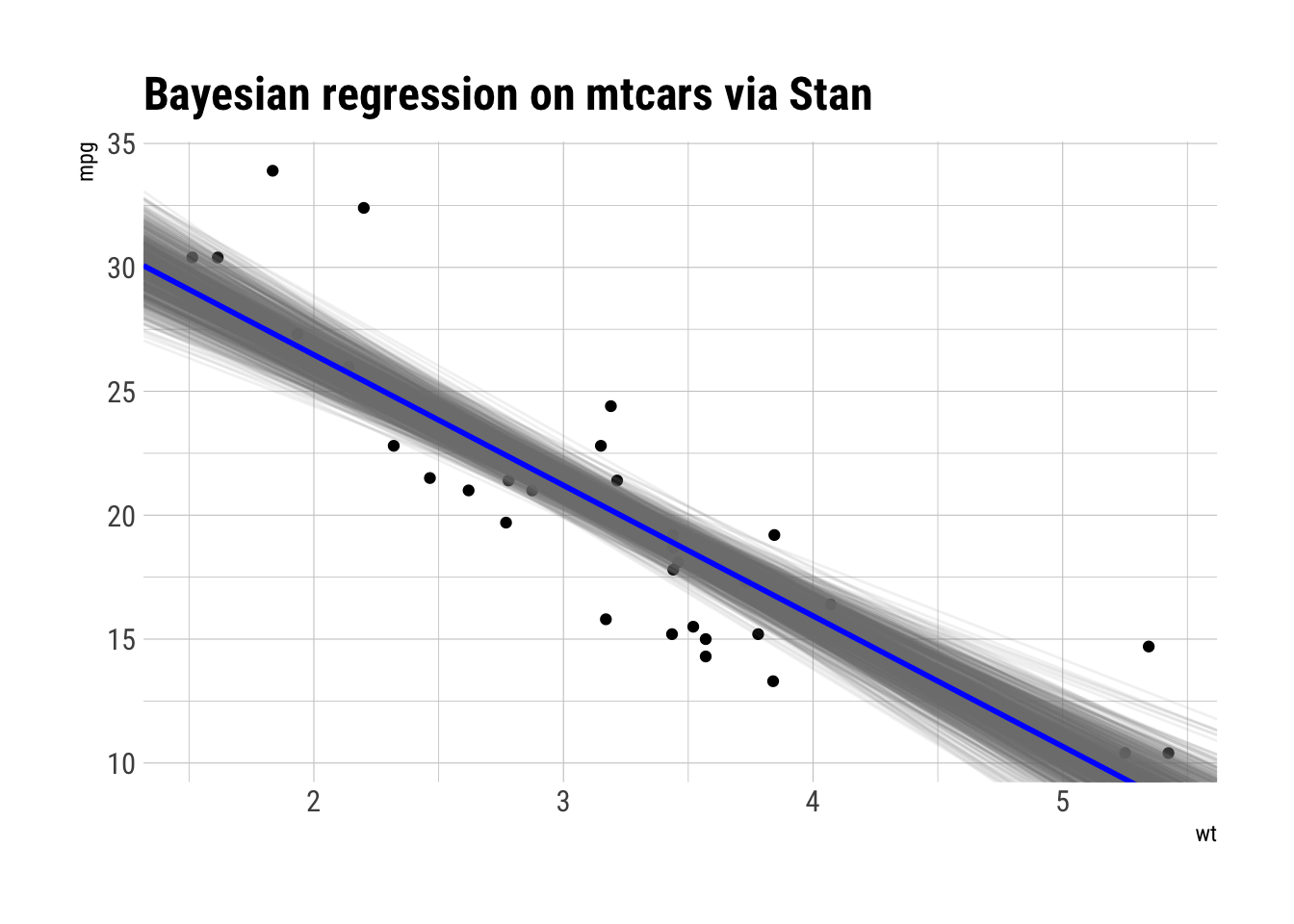
Looks quite plausible for the data at hand.
greta
Code for greta is very parallel to that of Stan, with the difference that code for a greta model is written entirely in R.
Input data is turned into a “greta array” object with as_data. Parameters are
defined with distribution functions similar to Stan, though in greta they also
produce greta arrays, albeit with not-yet-calculated data. There is no default
uninformative prior in greta, so we’ll insert some broad but plausible values.
library(greta)

x <- as_data(mtcars$wt)
y <- as_data(mtcars$mpg)

beta0 <- uniform(-100, 100)
beta1 <- uniform(-100, 100)
sigma <- uniform(0, 1000)

head(x)
#> greta array (operation)
#>
#>       [,1]
#> [1,] 2.620
#> [2,] 2.875
#> [3,] 2.320
#> [4,] 3.215
#> [5,] 3.440
#> [6,] 3.460

beta0
#> greta array (variable following a uniform distribution)
#>
#>      [,1]
#> [1,]  ?
To combine our greta arrays into a model, we use ordinary arithmetic, leaving
greta to keep track of array dimensions. We set our assumed distribution of the
output by assigning to the distribution function in a fashion akin to
names<-, but here setting our output distribution with our defined but
uncalculated arrays.
Once everything is defined, we pass the yet-uncalculated objects we want to get
out into the model function.
mu <- beta0 + beta1*x

distribution(y) <- normal(mu, sigma)

model_greta <- model(beta0, beta1, sigma)
None of the above objects individually look like much, but greta can use DiagrammeR to plot a beautiful dependency graph of the model:
plot(model_greta)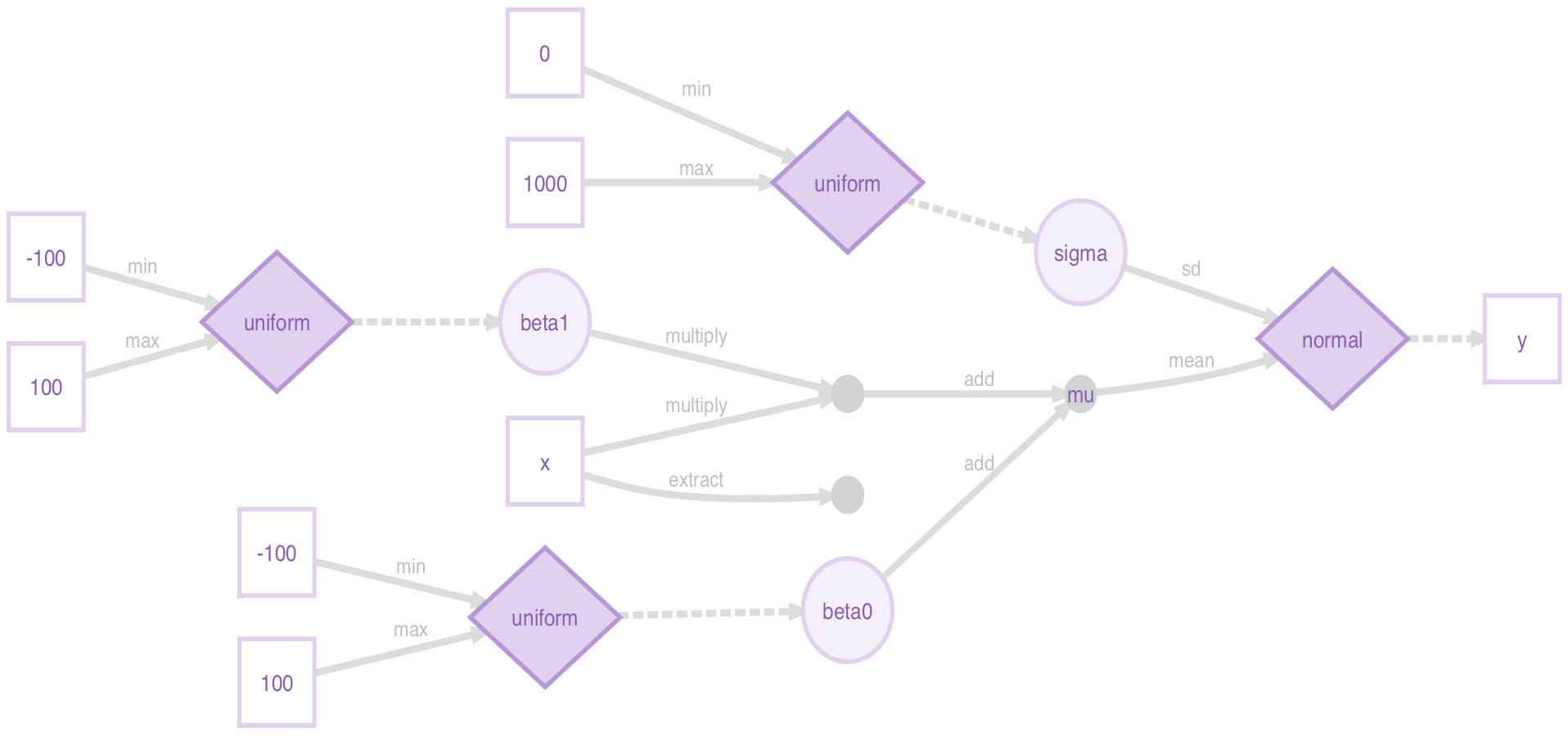
To actually run the simulations, we pass the model to the mcmc function. Here
I set the warmup and n_samples parameters to be parallel to Stan.
set.seed(47)

draws_greta <- mcmc(model_greta, warmup = 1000,  n_samples = 1000)
I am running this on my CPU, as the TensorFlow install is simpler. For such a small model, this is quite slow, taking about 2 minutes each for the warmup and sampling runs.2 It is supposed to scale well, though, so perhaps I am just running into overhead that will not grow or which would be much faster on more apt hardware. In any case, it does have a nice dynamic display showing the completed and remaining iterations and estimated time remaining, which seems pretty accurate, as progress bars go.
The resulting draws_greta object is a list of an array. It does not have a
useful print method, but its mcmc.list class (from
coda) does have nice
methods for summary and diagnostic plots:
summary(draws_greta)
#>
#> Iterations = 1:1000
#> Thinning interval = 1
#> Number of chains = 1
#> Sample size per chain = 1000
#>
#> 1. Empirical mean and standard deviation for each variable,
#>    plus standard error of the mean:
#>
#>         Mean     SD Naive SE Time-series SE
#> beta0 37.148 2.1323  0.06743        0.10598
#> beta1 -5.313 0.6399  0.02024        0.03252
#> sigma  3.154 0.4468  0.01413        0.06356
#>
#> 2. Quantiles for each variable:
#>
#>         2.5%    25%    50%    75%  97.5%
#> beta0 33.160 35.717 37.109 38.610 41.293
#> beta1 -6.536 -5.729 -5.319 -4.888 -4.105
#> sigma  2.345  2.864  3.113  3.374  4.248

bayesplot::mcmc_intervals(draws_greta)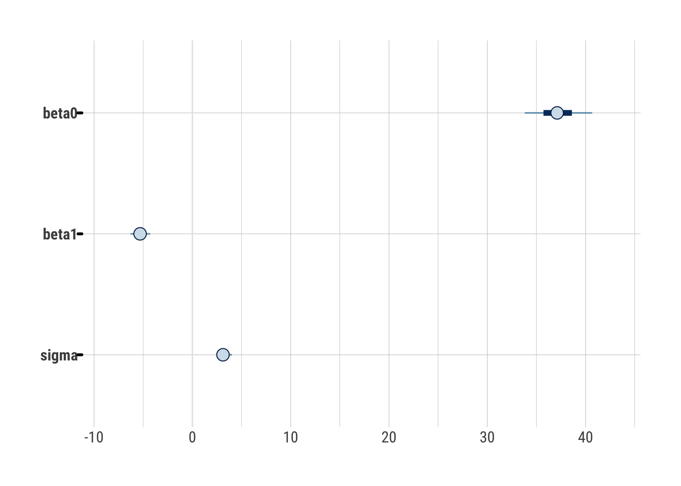
bayesplot::mcmc_trace(draws_greta)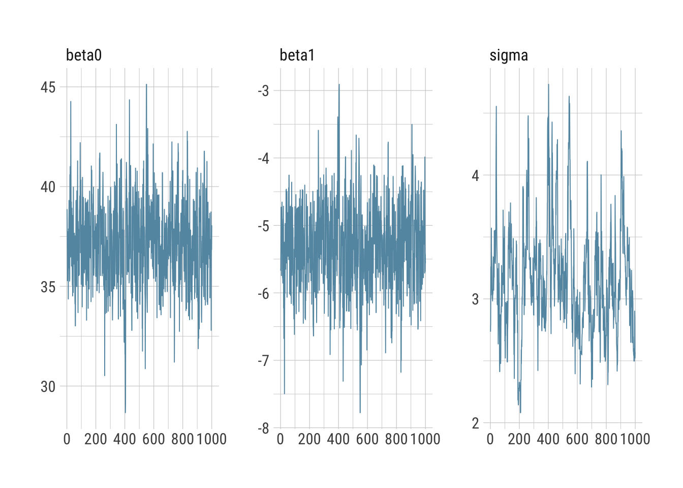
Everything looks reasonable and comparable to Stan.
Let’s extract and plot the results:
draws_greta_df <- as.data.frame(draws_greta[[1]])

ggplot(draws_greta_df, aes(beta0, beta1, color = sigma)) +
    geom_point(alpha = 0.3) +
    geom_density2d(color = "gray30") +
    scale_color_viridis_c(option = "plasma") +
    labs(title = "greta parameter space")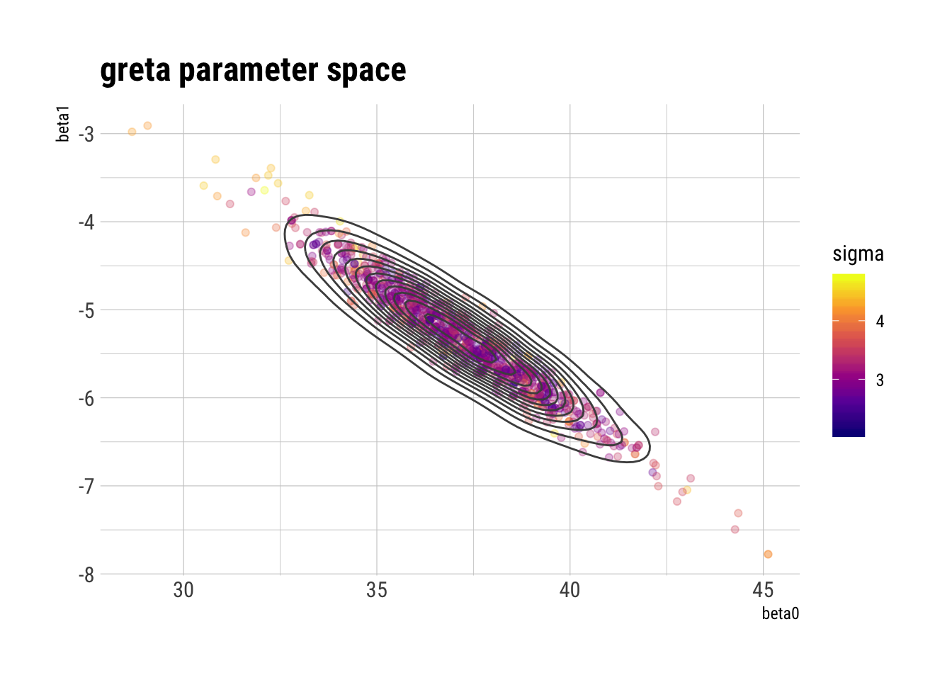
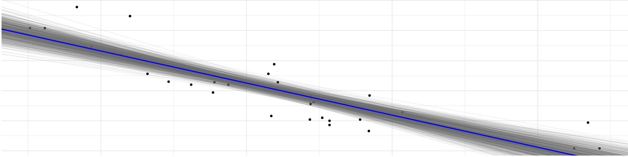
ggplot(mtcars, aes(wt, mpg)) +
    geom_point() +
    geom_abline(aes(intercept = beta0, slope = beta1), draws_greta_df,
                alpha = 0.1, color = "gray50") +
    geom_abline(slope = mean(draws_greta_df$beta1),
                intercept = mean(draws_greta_df$beta0),
                color = "blue", size = 1) +
    labs(title = "Bayesian regression on mtcars via greta")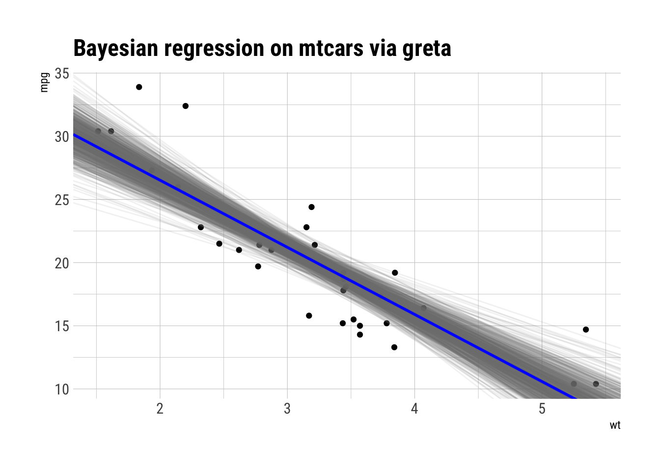
Looks pretty similar to Stan.
Reflections
Stan
Stan is actually another language, although it is not particularly complicated
or hard to learn. Since it is declarative imperative, it is easy to see
what goes where in the model, but not so easy to figure out where bugs are when
compilation fails. Error messages (aside from the annoying warnings) are pretty
good, though.
Written in an RMarkdown chunk, Stan is really easy to integrate into a larger
workflow without breaking stride. There is also the
rstanarm package, which assembles up typical
models into R functions. While this seems like it should be simpler, a quick
attempt showed it to actually be somewhat more finicky, as the resulting
functions have a lot of parameters and are fairly complicated compared to the
smaller, simpler individual pieces of stan itself.
The biggest problem I ran into is that since Stan is another language, the
documentation is not available with ?. In fact, it is
a 637-page PDF. The PDF is
in fact very well-written and organized, but still, it’s a PDF, which is
annoying as it does not integrate into the web well. (I can’t put a link to the
section on linear regression here.) Hopefully the documentation will eventually
be better integrated into the otherwise-great Stan website. In an ideal world,
it could be integrated into R’s help, too, though that would require some work.
greta
greta avoids a lot of the issues of Stan. Documentation is available as usual.
Intermediary products are easily viewable, and an individual problematic call
will fail, making debugging simpler. It is not quite as easy to look at the
code and quickly see the model structure, but the models plot method is a
pretty solution to this problem.
In terms of organization, greta almost unavoidably leaves a lot of objects in the global environment with no inherent organization. The objects will not fit neatly in a data frame, so there is no natural organizational approach. Everything could (and perhaps should) be kept in a list or environment. A more robust approach would be to make a class with slots for the parts of the model and a suitable print method. While more work to build and apply, such an approach would allow quicker manipulations of multiple models without mess or confusion.
The biggest drawback in my short experiment is speed. I ran simulations on slightly larger (not “big”, in any sense) data, and it had no effect on run time, which seems to be purely a function of the number of iterations. I am not sure how it scales, but given that it was explicitly built for such a purpose, hopefully what I experienced is just overhead.
Overall, greta is a bit less mature than Stan, which has a bigger, funded team working on it. Given that greta leverages other projects that have such an infrastructure, it may not require such dedicated resources, but it does have room to grow yet. Hopefully it will!
Bayesian simulation
For a relative beginner, both interfaces proved surprisingly simple and easily adaptable. I—as ever—have much yet to learn, but these frameworks will doubtlessly prove to be great assets with which to further explore the potential of Bayesian statistics.
h/t Daniel Lee. Thank you!↩
After upgrading to R 3.5.0 and reinstalling greta and TensorFlow, warmup and sampling take about 1 minute instead of 2. I’m not sure what caused the speedup, but it is wholly welcome!↩


Share this post