
Pythagorean Triples
The hidden patterns of right integer triangles
In a quiet moment, I happened across Project Euler’s Question 39:
Integer right triangles
Problem 39
If \(p\) is the perimeter of a right angle triangle with integral length sides, \(\{a,b,c\}\), there are exactly three solutions for \(p = 120\):
\[\{20,48,52\}, \{24,45,51\}, \{30,40,50\}\]
For which value of \(p \le 1000\), is the number of solutions maximised?
Put another way, what integer perimeter less than or equal to 1000 has the most Pythagorean triples?
While Wikipedia reveals there exist ways of generating triples directly like Euclid’s Formula, I find approaching Project Euler questions with the math I remember is decidedly more rewarding than simply implementing someone else’s solution, so I deliberately avoided searching for solutions, and got to coding.
The simplest possible solution would be some variation of iterating over integers the shorter leg \(a\) and longer leg \(b\) and checking if the hypotenuse \(c\) generated by the Pythagorean theorem \(c = \sqrt{a^2 + b^2}\) is an integer. In the course of implementing such an approach, some optimizations become obvious:
What are possible values for \(a\) and \(b\) to iterate over? Since the smallest triple is \(\{3, 4, 5\}\) and \(a < b < c\) (since the hypotenuse is longer than the legs and if \(a = b\) the triangle would be a 45-45-90 with \(c = a\sqrt{2}\)),
- \(a\) must be less than \(\frac{1}{3}P\) where \(P\) is the perimeter. Given the \(\{3, 4, 5\}\) and the question, \(12 \le P \le 1000\), so \(1 \le a \le 333\). The domain can actually be whittled further, but removing \(\frac{2}{3}\) of the cases is a solid start.
- Similarly, since \(b < c\), \(b\) makes up less than half of the perimeter, so \(2 \le b \le 499\).
More broadly, is iterating over \(a\) and \(b\) efficient, given the question is about perimeters? A more direct solution would be to iterate over \(P\) values. Each perimeter may have multiple triples, so nested iteration would still be necessary. But given \(P\), is one more parameter, e.g. \(c\), sufficient?
This last proposition seemed likely, and led me to explore on Desmos:
In this graph, \(x = a\), \(y = b\), \(c\) is parameterized as \(z\) (here iterating over integers from \(ceiling(\sqrt{2} - 1) * P\)—a right isosceles triangle— to \(\frac{P}{2}\)—a flat line), and the perimeter is another parameter \(P\) (here fixed at 120).
- The circle is the points for which the Pythagorean theorem holds, i.e. \(x^2 + y^2 = z^2\), i.e. right triangles.
- The black line is defined by \(P = a + b + c\), rearranged here as \(y = P - x - z\). As \(P\) and \(z\) are parameters that are fixed for any given value (here, frame), this equation therefore takes the form of a line with a slope of -1 and a y-intercept of \(P - z\).
- The violet area is defined by \(0 < x < y\), i.e. the only place solutions will exist.
Therefore, the intersection of the circle and the line within the violet region is the single right triangle for \(P = 120\) and the given \(z\) value. Obviously now, there is a single triangle for each perimeter and hypotenuse, though it is only a triple if all values are integers.
The graph also suggests how to solve for \(a\) and \(b\) for a given \(P\) and \(c\): solve the system of equations created by the perimeter and Pythagorean theorem for \(a\) or \(b\). Since \(P\) and \(c\) are constants, if solved for \(a\), then \(b\) is simply \(b = P - c - a\). Rearranging and substituting,
\[b = P - c - a = (P - c) - a\] \[a^2 + ((P - c) - a)^2 = c^2\] In terms of \(a\), this equation is a quadratic, so rearranging into standard form,
\[a^2 + (P - c)^2 + a^2 + 2(P - c)a = c^2\] \[2a^2 + 2(P - c)a + P^2 + 2Pc + c^2 = c^2\] \[2a^2 - 2(P - c)a + P(P - 2c)= 0\] While not exactly elegant, this is a quadratic where \(A = 2\), \(B = -2(P - c)\) and \(C = P(P - 2c)\), and thus can be solved for \(a\) using the quadratic formula:
\[a = \frac{2(P - c) \pm \sqrt{(-2(P - c))^2 - 4*2*P(P - 2c)}}{2 * 2}\] \[a = \frac{P - c \pm \sqrt{P^2 - 2Pc + c^2 - (2P^2 - 4Pc)}}{2}\] \[a = \frac{P - c \pm \sqrt{c^2 + 2Pc - P^2}}{2}\]
In fact, this equation shows how to solve for both \(a\) and \(b\); \(a\) will be the result of subtracting the discriminant, \(b\) adding (though subtracting from \(P\) is still simpler).
Best of all, coded in R, this equation is nicely vectorized across \(c\), so
legs <- function(P, c){
    discriminant <- sqrt(c^2 + 2*P*c - P^2)
    a <- (P - c - discriminant) / 2
    b <- P - c - a
    data.frame(a, b, c, P)
}

triples <- legs(120, 50:59)
triples
#>            a        b  c   P
#> 1  30.000000 40.00000 50 120
#> 2  24.000000 45.00000 51 120
#> 3  20.000000 48.00000 52 120
#> 4  16.699702 50.30030 53 120
#> 5  13.790627 52.20937 54 120
#> 6  11.139991 53.86001 55 120
#> 7   8.676192 55.32381 56 120
#> 8   6.355418 56.64458 57 120
#> 9   4.148557 57.85144 58 120
#> 10  2.035109 58.96489 59 120
Within this result are the three triples: \(\{30,40,50\}\), \(\{24,45,51\}\) and
\(\{20,48,52\}\), which can be separated by checking a %% 1 == 0:
triples[triples$a %% 1 == 0, ]
#>    a  b  c   P
#> 1 30 40 50 120
#> 2 24 45 51 120
#> 3 20 48 52 120
With this foundation, to generate triples for all \(P \le 1000\) just requires
iterating over \(P\). Optimized a bit and using purrr::map_dfr to collapse the
results,
triples <- purrr::map_df(12:1000, function(P){
    c <- seq.int(from = ceiling((sqrt(2) - 1) * P),    # 45-45-90
                 to = floor((P - 1) / 2),    # flat
                 by = 1L)
    discriminant <- sqrt(c^2 + 2*P*c - P^2)
    a <- (P - c - discriminant) / 2
    is_triple <- a %% 1 == 0
    if (any(is_triple)) {
        a <- a[is_triple]
        c <- c[is_triple]
        b <- P - c - a
        list(P = rep(P, length(a)),
             a = a,
             b = b,
             c = c)
    } else NULL
})

triples
#> # A tibble: 325 x 4
#>        P     a     b     c
#>    <int> <dbl> <dbl> <dbl>
#>  1    12    3.    4.    5.
#>  2    24    6.    8.   10.
#>  3    30    5.   12.   13.
#>  4    36    9.   12.   15.
#>  5    40    8.   15.   17.
#>  6    48   12.   16.   20.
#>  7    56    7.   24.   25.
#>  8    60   15.   20.   25.
#>  9    60   10.   24.   26.
#> 10    70   20.   21.   29.
#> # ... with 315 more rows
Beautiful. Answering the question from here is trivial, but more usefully, this approach has produced a lovely dataset to explore, and can easily produce an extended version by simply scaling to a bigger range of \(P\) values:
triples <- purrr::map_df(12:50000, function(P){
    c <- seq.int(from = ceiling((sqrt(2) - 1) * P),    # 45-45-90
                 to = floor((P - 1) / 2),    # flat
                 by = 1L)
    discriminant <- sqrt(c^2 + 2*P*c - P^2)
    a <- (P - c - discriminant) / 2
    is_triple <- a %% 1 == 0
    if (any(is_triple)) {
        a <- a[is_triple]
        c <- c[is_triple]
        b <- P - c - a
        list(P = rep(P, length(a)),
             a = a,
             b = b,
             c = c)
    } else NULL
})

triples
#> # A tibble: 29,933 x 4
#>        P     a     b     c
#>    <int> <dbl> <dbl> <dbl>
#>  1    12    3.    4.    5.
#>  2    24    6.    8.   10.
#>  3    30    5.   12.   13.
#>  4    36    9.   12.   15.
#>  5    40    8.   15.   17.
#>  6    48   12.   16.   20.
#>  7    56    7.   24.   25.
#>  8    60   15.   20.   25.
#>  9    60   10.   24.   26.
#> 10    70   20.   21.   29.
#> # ... with 29,923 more rows
Lovely. Let’s explore. After making a lot of plots, I found I mostly just wanted to try different aesthetics, so I wrote a function, coloring points by the parity of \(a\) to show some differentiation:
library(tidyverse)
#> ── Attaching packages ───────────────────────────────────────────────────────────── tidyverse 1.2.1 ──
#> ✔ ggplot2 2.2.1.9000     ✔ purrr   0.2.4
#> ✔ tibble  1.4.2          ✔ dplyr   0.7.4
#> ✔ tidyr   0.8.0          ✔ stringr 1.3.0
#> ✔ readr   1.2.0          ✔ forcats 0.3.0
#> ── Conflicts ──────────────────────────────────────────────────────────────── tidyverse_conflicts() ──
#> ✖ dplyr::filter() masks stats::filter()
#> ✖ dplyr::lag()    masks stats::lag()
#> ✖ dplyr::vars()   masks ggplot2::vars()

plot_triples <- function(aes,
                         ylab = rlang::quo_name(aes$y),
                         max_c = 20500){
    triples %>%
        filter(c < max_c) %>%    # subset if desired
        mutate(a_parity = ifelse(a %% 2 == 0, 'even', 'odd')) %>%
        ggplot(aes) +
        geom_point(size = 0.5, alpha = 0.5) +
        scale_x_continuous(labels = scales::comma_format(), expand = c(0, 0)) +
        scale_y_continuous(labels = scales::comma_format(), expand = c(0, 0)) +
        # prettify
        ggsci::scale_color_d3(
            guide = guide_legend(override.aes = list(alpha = 1))) +
        labs(title = 'Pythagorean Triples',
             y = ylab,
             color = expression(Parity~of~italic(a))) +
        hrbrthemes::theme_ipsum_rc(plot_margin = margin(10, 10, 5, 10),
                                   grid = FALSE) +
        theme(legend.position = 'bottom',
              legend.direction = 'horizontal',
              legend.key.size = unit(10, 'pt'),
              legend.justification = 0.01,
              legend.margin = margin(0, 0, 0, 0),
              axis.title.y = element_text(angle = 0))
}
Iterating plots is now quite quick. First, the relationship between \(a\) and \(b\), i.e. is the triangle long and skinny or near isosceles?
plot_triples(aes(b, a, color = a_parity), max_c = Inf)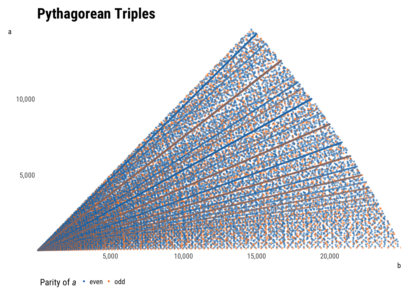
plot_triples(aes(b, a, color = a_parity))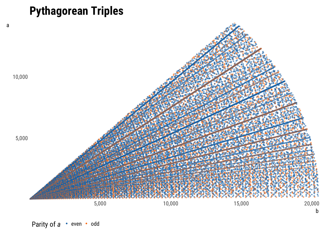
A few features are immediately apparent. Subsetting data by \(P\) (as it was generated) returns a triangle, which makes sense—if \(a\) is very small, \(b\) can claim more of the maximum perimeter, whereas if \(a\) is very large, the biggest \(b\) can be is a tiny bit larger. The tradeoff is linear, producing the upper-right leg of the triangle.
Subsetting by \(c\) instead turns the triangle into a sector of a circle. Taking the Pythagorean theorem as the equation of a circle, the shape makes sense. Unlimited, the graph would continue to the right.
The upper left leg or radius of the output space is the line \(y = x\), as \(a\) is defined as less than \(b\). If \(b\) were allowed to be larger than \(a\) (i.e. if the dataset were doubled by flipping \(a\) and \(b\)), this space would continues not only to the right, but also upwards through the rest of the first quadrant. Relaxing the assumption that \(a\) and \(b\) are positive would extend the space into all four quadrants. All non-plotted areas would be reflections of the current points.
More interesting than the output space are the patterns visible within the points. Most evident are the rays shooting out from the origin, which are explained by multiples: since \(\{3, 4, 5\}\) is a triple, \(\{6, 8, 10\}\), \(\{30, 40, 50\}\), etc. will be too. The densest rays are products of the smallest initial triples; spottier rays are products of larger initial triples that therefore recur less.
There are also some curvilinear patterns within the points. These are less simple to explain, but have been. They are parabolas centered along each axis with foci at the origin.
Let’s get some different views.
plot_triples(aes(c, a, color = a_parity))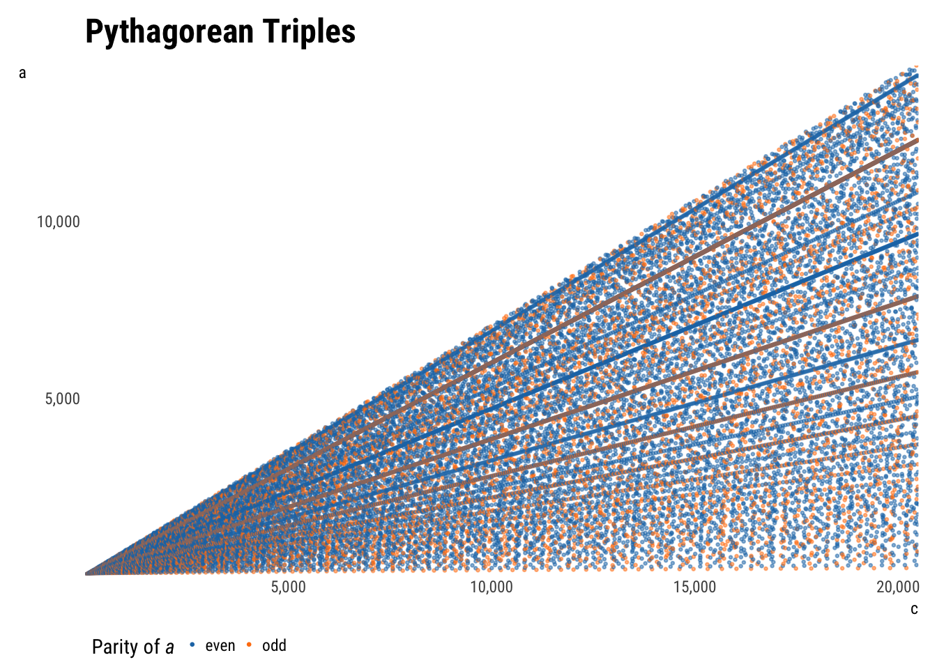
Plotting \(a\) as a function of \(c\) instead of \(b\), the rays remain, but the parabolas change. The concavity of one set has flipped, and the other has turned into diagonal lines.
Curious. Let’s rearrange.
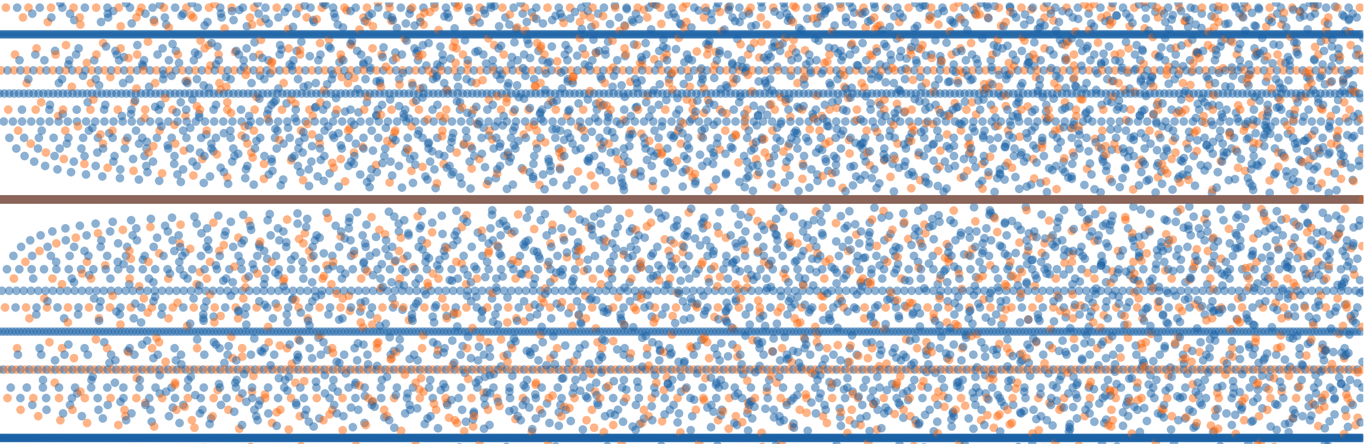
plot_triples(aes(c, a/c, color = a_parity),
             ylab = expression(over(a, c)))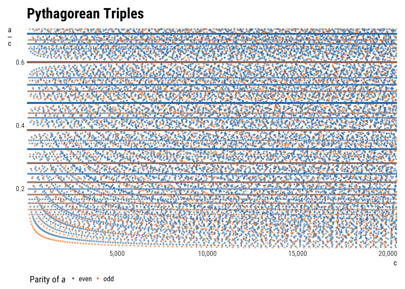
This is the same as the plot above, but with \(a\) rescaled by \(c\) so as to spread the rays converging at the origin across the y-axis. The multiples are now more easily identifiable: for \(\{3, 4, 5\}\), \(\frac{a}{c}=\frac{3}{5}=0.6\).
The diagonal lines have been turned into hyperbolas à la \(y = \frac{1}{x}\) now, which is a sensible result of dividing by the x variable.
Another exciting effect is the empty space by where each multiple line meets y-axis. It is explicable: to get a triple with a \(\frac{a}{c}\) ratio close to 0.6 without using a multiple of \(\frac{3}{5}\) requires a reasonably large denominator. Harder to explain is the continued rarefaction of the space further across the graph, particularly visible for the 0.6 line.
Find another pattern? Let me know!

Share this post